👩🏼‍🏫 Math285 midterm review

First Order ODE

Approach

To solve $y' = a(t)y + b(t)$ :

1. Find $A(t)$: Calculate the integral of $a(t)$: $A(t) = \int a(t) \, dt$. You can ignore the constant of integration for this step.

2. Calculate $e^{A(t)}$ and $e^{-A(t)}$: Compute the exponential of $A(t)$ and its negative.

3. Find the Integral Part: Calculate the integral of $b(t) \cdot e^{-A(t)}$: $\int b(t)e^{-A(t)} \, dt$. Let’s call the result of this integral $I(t)$.

4. Particular Solution: A particular solution is given by $y_p(t) = e^{A(t)} \cdot I(t)$.

5. General Solution: The general solution is $y(t) = c \cdot e^{A(t)} + y_p(t)$, where $c$ is an arbitrary constant.

Sample

1 For the solution $y(t)$ of the IVP $y' = (y/t) - 1$, $y(1) = \ln 2$, the value $y(2)$ is equal to:

• 0
• 1
• 2
• $\ln 2$
• $2\ln 2$

2. For the solution $y(t)$ of the IVP $y' = \frac{ty+1}{t^2+1}$, $y(0) = 2$, the value $y(1)$ is equal to:

• $\sqrt{2}$
• 2
• $1+\sqrt{2}$
• 3
• $1+2\sqrt{2}$

3. For the solution $y(t)$ of the IVP $y' = \frac{2y+1}{t}$, $y(1) = 2$, the value $y(2)$ is equal to:

• 11/2
• 13/2
• 15/2
• 17/2
• 19/2

Separatble ODEs

Approach

Given a separable ODE of the form: $\frac{dy}{dt} = f(t)g(y)$

1. Separate: $\frac{dy}{g(y)} = f(t) dt$

2. Integrate: $\int \frac{1}{g(y)} dy = \int f(t) dt$

   Let $G(y) = \int \frac{1}{g(y)} dy$ and $F(t) = \int f(t) dt$

   Then, the equation becomes: $G(y) = F(t) + C$ (where $C$ is the integration constant)

3. Apply Initial Condition $y(t_0) = y_0$: $G(y_0) = F(t_0) + C$

4. Solve for $C$: $C = G(y_0) - F(t_0)$

5. Specific Solution (Implicit Form): $G(y) = F(t) + G(y_0) - F(t_0)$

6. Solve for $y$ (Explicit Form - if possible): If possible, solve $G(y) = F(t) + C$ (or $G(y) = F(t) + G(y_0) - F(t_0)$) for $y$ to get $y = h(t, C)$ or $y = h(t, t_0, y_0)$.

7. Evaluate $y(t_1)$: Substitute $t = t_1$ into the explicit solution $y = h(t, C)$ (or implicit solution and solve for $y$) to find $y(t_1)$.

Sample

1. For the solution $y(t)$ of the IVP $y' = y\ln t$, $y(1) = 1$ the value $y(e)$ is equal to

   • $e^{-2}$
   • $e^{-1}$
   • 1
   • $e$
   • $e^{2}$

2. For the solution $y(t)$ of the IVP $y' = y^2e^{-t}$, $y(0) = -1$ the value $y(-1)$ is equal to

   • $e$
   • $1/(e-2)$
   • $e+2$
   • $1/(e+2)$
   • $e-2$

3. For the solution $y(t)$ of the IVP $y' = e^{t-2y}$, $y(0) = 0$ the value $y(1)$ is contained in

   • $[0, \frac{1}{2}]$
   • $[\frac{1}{2}, 1]$
   • $[1, \frac{3}{2}]$
   • $[\frac{3}{2}, 2]$
   • $[2, \infty)$

4. For the solution $y(t)$ of the IVP $y' = (y^2-3)/(ty)$, $y(1) = 2$ the value $y(2)$ is equal to

   • $\sqrt{6}$
   • $\sqrt{7}$
   • $\sqrt{8}$
   • $3$
   • $\sqrt{10}$

5. For the solution $y(t)$ of the IVP $y' = -t(y^2+1)$, $y(0) = 1$ the value $y(1)$ is contained in

   • $[0, \frac{1}{2}]$
   • $[\frac{1}{2}, 1]$
   • $[1, \frac{3}{2}]$
   • $[\frac{3}{2}, 2]$
   • $[2, \infty)$

Exact Differential Equations and Integrating Factors

Approach

Goal: Find integrating factor $\mu$ for ODE $M dx + N dy = 0$

Exactness Check: Is $M_y = N_x$? If yes, ODE is exact.

Integrating Factor Cases:

$\mu$ Type	Condition for $g$	Formula for $g$	Case No.	$\mu'(s) = $ Relation
$\mu(x)$	$\frac{M_y - N_x}{N} = g(x)$	$\frac{M_y - N_x}{N}$	①	$\mu'(s) = g(s)\mu(s)$
$\mu(y)$	$\frac{M_y - N_x}{-M} = g(y)$	$\frac{M_y - N_x}{-M} = \frac{N_x - M_y}{M}$	②	$\mu'(s) = -g(s)\mu(s)$
$\mu(xy)$	$\frac{M_y - N_x}{N_y - M_x} = g(xy)$	$\frac{M_y - N_x}{N_y - M_x}$	③	$\mu'(s) = g(s)\mu(s)$
$\mu(\frac{y}{x})$	$\frac{x^2(M_y - N_x)}{N_y + M_x} = g(\frac{y}{x})$	$\frac{x^2(M_y - N_x)}{N_y + M_x}$	④	$\mu'(s) = -g(s)\mu(s)$

Note:

• After finding the correct case and $g(s)$, calculate $\mu(s)$ by solving the $\mu'(s) = \pm g(s)\mu(s)$ relationship which leads to $\mu(s) = e^{\pm \int g(s) ds}$.
• Multiply the original ODE by $\mu$ to make it exact.

Sample

1. The ODE $(y^2 + y) dx - x dy$ has the integrating factor

   • 0
   • $x^{-1}$
   • $y^{-1}$
   • $x^{-2}$
   • $y^{-2}$

2. The ODE $(x^4y^2 - y) dx + (x^2y^4 - x) dy = 0$ has the integrating factor

   • $1/(xy)$
   • 1
   • $1/(xy)^2$
   • $1/(xy^2)$
   • $1/(x^2y)$

3. The family of curves $y = c/x^2, c \in \mathbb{R}$ satisfies the ODE

   • $dy = x^{-2} dx$
   • $dy = 2x^{-3} dx$
   • $2xy dx + x^2 dy = 0$
   • $dx = dy$
   • $2yx^{-3} dx - x^{-2} dy = 0$

4. The ODE $3x dx - (y - 3x^2/y) dy$ has the integrating factor

   • 0
   • $x$
   • $y$
   • $x^2$
   • $y^2$

Radius of Convergence

Approach

To find the radius of convergence $R$ of a power series $\sum_{n=0}^{\infty} c_n z^n$:

1. Find the Coefficients:

   • Identify the coefficients $c_n$ in your power series. This is the number multiplying $z^n$. Look for a pattern in these numbers as $n$ changes (0, 1, 2, 3…).
   • Important for series with “gaps”: If some powers of $z$ are missing (like $z^3, z^5$ are present but $z^2, z^4$ are not), the coefficient for the missing power is zero. You need to define $c_n$ for all $n \ge 0$.

2. Calculate $|c_n|^{1/n}$ (or Estimate Its Limit):

   • Take the absolute value of each coefficient $|c_n|$.
   • Raise it to the power of $1/n$ (which is the same as taking the $n$-th root: $\sqrt[n]{|c_n|}$).
   • Think about what happens to $|c_n|^{1/n}$ as $n$ becomes very large. What is the limit as $n \to \infty$? Let’s call this limit $L$. In many simple cases, you can just estimate this limit.

3. Find the Limit Superior $L = \limsup_{n \to \infty} (|c_n|^{1/n})$ (More precisely):

   • For more complicated series, or if the limit from step 2 is not obvious, you might need to find the limit superior. But often for introductory problems, the simple limit from step 2 works. Assume for now that $L = \lim_{n \to \infty} (|c_n|^{1/n})$ exists.

4. Calculate Radius $R$:

   • Once you have $L$, the radius of convergence $R$ is:
     • If $L > 0$, then $R = \frac{1}{L}$.
     • If $L = 0$, then $R = \infty$ (series converges for all $z$).
     • If $L = \infty$, then $R = 0$ (series only converges for $z = 0$).

Simplified Steps (Formula Focus):

1. Get $c_n$: Identify the coefficient of $z^n$.
2. Calculate $|c_n|^{1/n}$: Compute the $n$-th root of the absolute value of $c_n$.
3. Find $L = \lim_{n\to\infty} |c_n|^{1/n}$ (or $\limsup$).
4. Radius $R$:
   • $R = 1/L$, if $0 < L < \infty$
   • $R = \infty$, if $L = 0$
   • $R = 0$, if $L = \infty$

Sample

1. The power series $z + \frac{1}{2}z^2 + \frac{1}{4}z^4 + \frac{1}{8}z^8 + \frac{1}{16}z^{16} + \dots$ has radius of convergence

   • 0
   • 1
   • $\sqrt{2}$
   • 2
   • $\infty$

2. The power series $\sum_{k=1}^{\infty} 2^{k}z^{k^2}$ has radius of convergence

   • 0
   • $\frac{1}{2}$
   • 1
   • 2
   • $\infty$

3. The power series $z + z^2 + z^4 + z^8 + z^{16} + \dots$ has radius of convergence

   • 0
   • $\frac{1}{2}$
   • 1
   • 2
   • $\infty$

Picard-Iteration

Approach

Problem-Solving Approach for Picard-Lindelöf Iterates

To find $\phi_2(t)$ (the second Picard-Lindelöf iterate) for an Initial Value Problem (IVP) using the iterative formula:

$\phi_{k+1}(t) = y_0 + \int_{0}^{t} f(s, \phi_k(s)) \, ds, \quad k = 0, 1, 2, \dots$

Steps:

1. Identify $f(t, y)$ and $y_0$ from the IVP: For an IVP in the form $y' = f(t, y)$, $y(0) = y_0$, determine the function $f(t, y)$ and the initial value $y_0$.

2. Determine the Initial Iteration $\phi_0(t)$: The starting point for the iteration is the constant function based on the initial condition: $\phi_0(t) = y_0$

3. Calculate the First Iteration $\phi_1(t)$ (for k=0 in the formula): Use the formula with $k=0$: $\phi_1(t) = y_0 + \int_{0}^{t} f(s, \phi_0(s)) \, ds$ Substitute $\phi_0(s) = y_0$ into $f(s, \phi_0(s))$, then evaluate the definite integral with respect to $s$ from $0$ to $t$.

4. Calculate the Second Iteration $\phi_2(t)$ (for k=1 in the formula): Use the formula with $k=1$: $\phi_2(t) = y_0 + \int_{0}^{t} f(s, \phi_1(s)) \, ds$ Substitute the expression you found for $\phi_1(s)$ into $f(s, \phi_1(s))$, then evaluate the definite integral with respect to $s$ from $0$ to $t$.

5. Select the Correct Option: Compare your calculated expression for $\phi_2(t)$ with the provided multiple-choice options and choose the one that matches.

Formula-Based Steps Summary:

1. Identify: $f(t,y), y_0$ from $y' = f(t, y), y(0) = y_0$
2. Set: $\phi_0(t) = y_0$
3. Calculate $\phi_1(t)$: $\phi_1(t) = y_0 + \int_{0}^{t} f(s, \phi_0(s)) \, ds$
4. Calculate $\phi_2(t)$: $\phi_2(t) = y_0 + \int_{0}^{t} f(s, \phi_1(s)) \, ds$
5. Match: Compare $\phi_2(t)$ to options.

Important Note: The integral is always evaluated from $0$ to $t$, and in each step you’re substituting the previous iterate into the function $f$. You are iteratively refining an approximation to the solution of the IVP.

Sample

1. The sequence $\phi_0, \phi_1, \phi_2, \dots$ of Picard-Lindelöf iterates for the IVP $y' = y+t$, $y(0) = -1$ has $\phi_2(t)$ equal to

   • $\frac{1}{6}t^3$
   • $-1 - t - \frac{1}{2}t^2$
   • $-1 - t + \frac{1}{6}t^3$
   • $-1 - t - \frac{1}{2}t^2 + \frac{1}{6}t^3$
   • $-1 - t$

2. The sequence $\phi_0, \phi_1, \phi_2, \dots$ of Picard-Lindelöf iterates for the IVP $y' = y+2t$, $y(0) = -2$ has $\phi_2(t)$ equal to

   • $-2 + 2t + \frac{1}{3}t^3$
   • $-t^2 + \frac{1}{3}t^3$
   • $-2 - 2t + \frac{1}{3}t^3$
   • $t^2 + \frac{1}{3}t^3$
   • $1 + t + \frac{3}{2}t^2 + \frac{1}{3}t^3$

3. The sequence $\phi_0, \phi_1, \phi_2, \dots$ of Picard-Lindelöf iterates for the IVP $y' = 2y+2$, $y(0) = 2$ has $\phi_2(t)$ equal to

   • $2t + 6t^2$
   • $2t + 5t^2$
   • $2 + 6t + 6t^2$
   • $2t + 4t^2$
   • $1 + 4t + 4t^2$

Matrix Norms

Approach

For a matrix $A$, the norm of $A$ can be defined in different ways. Two common matrix norms are the Operator Norm ($||A||$) and the Frobenius Norm ($||A||_F$).

1. Operator Norm ($||A||$) - (Subordinate to Euclidean length)

• Definition (using unit vectors parameterized by trigonometric functions):

  Let $x = \begin{pmatrix} \sin x \\ \cos x \end{pmatrix}$, where $x \in [0, 2\pi]$. This $x$ represents any vector on the unit circle in $\mathbb{R}^2$. The Operator Norm of $A$ is defined as:$||A|| = \max \{||Ax||_2 \}$

  where $||Ax||_2$ is the Euclidean norm (length) of the vector $Ax$. This means we find the maximum length of the vector $Ax$ when $x$ is a unit vector.

• Example Calculation for $A = \begin{pmatrix} \frac{1}{2} & \pm 1 \\ 0 & \frac{1}{2} \end{pmatrix}$ :

  Using $x = \begin{pmatrix} \sin x \\ \cos x \end{pmatrix}$, calculate $||Ax||_2$:

  $||A|| = \max_{x} \left\{ \left\| \begin{pmatrix} \frac{1}{2} & \pm 1 \\ 0 & \frac{1}{2} \end{pmatrix} \begin{pmatrix} \sin x \\ \cos x \end{pmatrix} \right\|_2 \right\}$

  $ = \max_{x} \left\{ \left\| \begin{pmatrix} \frac{1}{2} \sin x \pm \cos x \\ \frac{1}{2} \cos x \end{pmatrix} \right\|_2 \right\}$

  $ = \max_{x} \left\{ \sqrt{ \left( \frac{1}{2} \sin x \pm \cos x \right)^2 + \left( \frac{1}{2} \cos x \right)^2 } \right\}$

  $ = \sqrt{ \frac{3}{4} + \frac{\sqrt{2}}{2} } = \frac{1 + \sqrt{2}}{2} \approx 1.207 $

2. Frobenius Norm ($||A||_F$):

• Definition:

  The Frobenius Norm of a matrix $A$ is defined as the square root of the sum of the squares of all its elements:$||A||_F = \sqrt{ \sum_{i,j} |a_{ij}|^2 }$

  This is essentially calculating the Euclidean norm of the matrix treated as a vector.

• Example Calculation for $A = \begin{pmatrix} \frac{1}{2} & \pm 1 \\ 0 & \frac{1}{2} \end{pmatrix}$ :

  $||A||_F = \sqrt{ \left(\frac{1}{2}\right)^2 + (\pm 1)^2 + (0)^2 + \left(\frac{1}{2}\right)^2 }$

  $ = \sqrt{ \frac{1}{4} + 1 + 0 + \frac{1}{4} } $

  $ = \sqrt{ \frac{1}{2} + 1 } = \sqrt{ \frac{3}{2} } = \frac{\sqrt{6}}{2} \approx 1.225 $

Sample

1. The matrix norm of $\begin{pmatrix} 2 & -3 \\ 3 & 2 \end{pmatrix}$ (subordinate to the Euclidean length on $\mathbb{R}^2$) is contained in the interval

   • $[1, 2]$
   • $[2, 3]$
   • $[3, 4]$
   • $[4, 5]$
   • $[5, 6]$

2. The matrix norm of $\begin{pmatrix} 1 & -1 \\ 1 & 1 \end{pmatrix}$ (subordinate to the Euclidean length on $\mathbb{R}^2$) is equal to

   • 0
   • 1
   • $\sqrt{2}$
   • 2
   • 4

3. The matrix norm of $\begin{pmatrix} 2 & 1 \\ 1 & 0 \end{pmatrix}$ (subordinate to the Euclidean length on $\mathbb{R}^2$) is equal to

   • 0
   • 1
   • $\sqrt{2}$
   • 2
   • $1+\sqrt{2}$

Phase Line

1. Basic Concepts

• Autonomous Equation: A differential equation \( y' = f(y) \) that depends only on the variable \( y \) and does not explicitly contain the independent variable \( t \).
• Equilibrium Points: The values of \( y \) that make \( f(y) = 0 \), which are critical points where the solution remains constant.
• Phase Line: A representation on the \( y \)-axis that marks equilibrium points and analyzes the sign of \( y' \) in their vicinity to determine the increasing or decreasing trend of solutions.

---

2. Steps of Phase Line Analysis

(1) Find Equilibrium Points

Solve the equation \( f(y) = 0 \) to obtain all equilibrium points \( y = c_1, c_2, \dots \).

(2) Divide into Intervals

Divide the \( y \)-axis into several intervals using the equilibrium points as dividers. For example, if equilibrium points are \( y = -2, 0, 2 \), the intervals are:

\[ (-\infty, -2),\ (-2, 0),\ (0, 2),\ (2, +\infty) \]

(3) Analyze the Sign of the Derivative

In each interval, choose any point \( y_0 \) and substitute it into \( f(y) \) to calculate the sign of \( y' \):

• If \( y' > 0 \), the solution is increasing in this interval (arrow points to the right).
• If \( y' < 0 \), the solution is decreasing in this interval (arrow points to the left).

(4) Determine Stability of Equilibrium Points

• Stable: If arrows on both sides point towards the equilibrium point (e.g., \( \rightarrow \leftarrow \)).
• Unstable: If arrows on both sides point away from the equilibrium point (e.g., \( \leftarrow \rightarrow \)).
• Semi-stable: If on one side the arrow points towards, and on the other side it points away (e.g., \( \rightarrow \rightarrow \) or \( \leftarrow \leftarrow \)).

---

3. Application Examples

Example 1: \( y' = y^4 - 4y^2 \), initial value \( y(4.29) = 1 \)

1. Equilibrium Points: Solve \( y^4 - 4y^2 = 0 \), yielding \( y = -2, 0, 2 \).
2. Sign of Derivative in Intervals:
   • \( y > 2 \): \( y' = (+) \) (increasing, arrow to the right).
   • \( 0 < y < 2 \): \( y' = (-) \) (decreasing, arrow to the left).
   • \( -2 < y < 0 \): \( y' = (+) \) (increasing, arrow to the right).
   • \( y < -2 \): \( y' = (-) \) (decreasing, arrow to the left).
3. Stability:
   • \( y = -2 \): Stable (arrows on both sides point towards it).
   • \( y = 0 \): Semi-stable (right arrow points left, left arrow points right).
   • \( y = 2 \): Unstable (arrows on both sides point away).
4. Solution Trend: Initial value \( y = 1 \) is in \( (0, 2) \), \( y' < 0 \), solution is decreasing and trends towards \( y = 0 \). Limit: \(\boxed{0}\)

Example 2: \( y' = y^3 - 7y + 6 \), initial value \( y(0) = 0 \)

1. Equilibrium Points: Solve \( y^3 - 7y + 6 = 0 \), yielding \( y = -3, 1, 2 \).
2. Sign of Derivative in Intervals:
   • \( y > 2 \): \( y' = (+) \).
   • \( 1 < y < 2 \): \( y' = (-) \).
   • \( -3 < y < 1 \): \( y' = (+) \).
   • \( y < -3 \): \( y' = (-) \).
3. Stability:
   • \( y = -3 \): Unstable.
   • \( y = 1 \): Stable.
   • \( y = 2 \): Unstable.
4. Solution Trend: Initial value \( y = 0 \) is in \( (-3, 1) \), \( y' > 0 \), solution is increasing and trends towards \( y = 1 \). Limit: \(\boxed{1}\)

Example 3: \( y' = y^4 - 1 \), initial value \( y(2021) = 0 \)

1. Equilibrium Points: Solve \( y^4 - 1 = 0 \), yielding \( y = -1, 1 \).
2. Sign of Derivative in Intervals:
   • \( y > 1 \): \( y' = (+) \).
   • \( -1 < y < 1 \): \( y' = (-) \).
   • \( y < -1 \): \( y' = (+) \).
3. Stability:
   • \( y = -1 \): Stable.
   • \( y = 1 \): Unstable.
4. Solution Trend: Initial value \( y = 0 \) is in \( (-1, 1) \), \( y' < 0 \), solution is decreasing and trends towards \( y = -1 \). Limit: \(\boxed{-1}\)

Second Order ODE (homogenous and inhomogenous)

$ay'' + by' + cy = r(x)$

where $a$, $b$, $c$ are constants, and $r(x)$ is a function of $x$.

Homogenous Second Order ODEs: $ay'' + by' + cy = 0$

1. Write down the Characteristic Equation: $ar^2 + br + c = 0$

2. Solve the Characteristic Equation:

   • Find the roots $\alpha_1, \alpha_2$ of this quadratic equation using the formula: $\alpha_{1,2} = \dfrac{-r_1 \pm \sqrt{r_1^2 - 4r_0}}{2}$

3. Check Root Type:

   A. Distinct Roots ($\alpha_1 \neq \alpha_2$, when $r_1^2 \neq 4r_0$)

   1. Real Distinct Roots

      • General Solution: $y = C_1 e^{\alpha_1 t} + C_2 e^{\alpha_2 t}$

   2. Complex Conjugate Roots ($\alpha_{1,2} = \zeta \pm i\beta$)

      • General Solution: $y = e^{\zeta t}(C_1 \cos(\beta t) + C_2 \sin(\beta t))$

   B. Repeated Roots ($\alpha_1 = \alpha_2 = \alpha$, when $r_1^2 = 4r_0$)

   • General Solution: $y = C_1 e^{\alpha t} + C_2 t e^{\alpha t}$

Note: In all cases, $C_1$ and $C_2$ are arbitrary constants determined by initial conditions.

Inhomogeneous Second Order ODEs: $ay'' + by' + cy = r(x)$

This section details the “Method of Undetermined Coefficients” (待定系数法) to find a particular solution $y_p(x)$ for the inhomogeneous equation.

1. Choosing the Form of $y_p(x)$ - Based on r(x)

The choice of the form of the particular solution $y_p(x)$ depends on the form of the function $r(x)$. Use the following table as a guide:

Term in r(x)	Choice for $y_p(x)$
$ke^{γx}$	$Ce^{γx}$
$kx^n$ (n = 0, 1, …)	$K_nx^n + K_{n-1}x^{n-1} + ... + K₁x + K₀$
$k \cos ωx$	$K \cos ωx + M \sin ωx$
$k \sin ωx$	$K \cos ωx + M \sin ωx$
$ke^{αx} \cos ωx$	$e^{αx} (K \cos ωx + M \sin ωx)$
$ke^{αx} \sin ωx$	$e^{αx} (K \cos ωx + M \sin ωx)$

where $k, γ, n, ω, α$ are known constants, and $C, K_i, M$ are undetermined coefficients that need to be determined by substituting $y_p(x)$ into the ODE.

2. Rules for Determining $y_p(x)$

• Basic Rule : If $r(x)$ consists of terms listed in the table above, then choose $y_p(x)$ to have the corresponding form from the “Choice for $y_p(x)$” column and solve for the undetermined coefficients.

• Modification Rule : If a term in the initially chosen $y_p(x)$ is already a solution to the corresponding homogeneous ODE ($ay'' + by' + cy = 0$), modify the choice for $y_p(x)$ by multiplying it by $x$ (or by $x^s$ if necessary, where $s$ is the smallest positive integer that makes no term in the modified $y_p(x)$ a solution to the homogeneous equation. Usually, multiplication by $x$ or $x^2$ is sufficient).

• Sum Rule : If $r(x)$ is a sum of several terms, the particular solution $y_p(x)$ should be taken as the sum of the particular solutions corresponding to each term in $r(x)$, adjusting each component with the Modification Rule if needed.

---

Basic Rule: 若 $r(x)$ 包含在上表左列中，那么 $y_p(x)$ 就取右侧对应的形式，之后代入求系数

Modification Rule: 若使用Basic Rule选取的 $y_p(x)$ 是（6.1）对应的齐次ODE的解时，取 $y_p(x)$ 与 $x$ 的乘积生成新的 $y_p(x)$ (若齐次ODE有重根复、 且 $y_p(x)$ 就是那个根时， 乘以的是 $x^2$ )

Sum Rule: 若 $r(x)$ 是上表左列几种情况的加和， 那么 $y_p(x)$ 也是右侧对应的几种情况的加和， 注意，加和前根据Modification Rule对每项进行调整。

---

3. Example: Find the General Solution of $y'' - y = 16e^{-x}$

STEP1: Solve the corresponding homogeneous equation y’’ - y = 0. The characteristic equation is $r^2 - 1 = 0 \Rightarrow r = \pm 1$. Therefore, the complementary function is

$y_c(x) = c_1e^x + c_2e^{-x}$

STEP2: According to the table, assume $y_p(x) = Be^{-x}$. However, because it duplicates a term from the complementary function, according to the Modification Rule, we need to multiply by an $x$, so assume $y_p(x) = Bxe^{-x}$.

STEP3: Substitute into the original equation, solve for coefficients.

$16e^{-x} = y_p'' - y_p = B(x - 2)e^{-x} - (Bxe^{-x}) = -2Be^{-x}$ $\Rightarrow B = -8 \Rightarrow y_p(x) = -8xe^{-x}$

Final general solution for y(x) is $y(x) = -8xe^{-x} + c_1e^x + c_2e^{-x}$

---

补充点稀奇古怪的知识

零化算子法（Method of Annihilators）

核心思想：通过构造一个能“零化”非齐次项的微分算子，将原非齐次方程转化为高阶齐次方程，从而确定特解的形式。

1. 确定零化算子：
   针对非齐次项 $f(x)$ 的类型选择相应的微分算子 $L$，使得$L[f(x)] = 0$。

   • 若 $f(x) = P_n(x)e^{\alpha x}$（其中 $P_n(x)$ 为 $n$ 次多项式），则零化算子为 $(D - \alpha)^{n+1}$。
   • 例如：若 $f(x) = 2xe^x$，则零化算子为 $(D - 1)^2$.

2. 构造高阶齐次方程：
   将零化算子作用于原方程两边，得到新的齐次方程： $(D - 1)^2 \cdot (D^2 - 3D + 2)y = 0$。
   其对应的特征根为原方程的根（$\lambda = 1,\,2$）以及零化算子引入的重根（$\lambda = 1$ 三重根）。

3. 确定特解形式：
   新齐次方程的通解形式为：$y = (C_1 + C_2x + C_3x^2)e^x + C_4e^{2x}$。
   从中选取与原齐次解 $y_h = C_1e^x + C_2e^{2x}$
   线性无关的部分作为特解形式： $y^* = x(Ax + B)e^x = Ax^2e^x + Bxe^x$.

4. 代入原方程求系数：
   将 $y^*$ 代入原方程 $y'' - 3y' + 2y = 2xe^x$， 通过比较系数解出 $A = -2,\quad B = -1$，
   最终特解为：$y^* = -2x^2e^x - xe^x$.

微分算子法(used in final exam)

算了写final里面了

Euler Equation

Approach

Equation Form: $ax^2y'' + bxy' + cy = 0$

Steps:

1. Characteristic Equation: Substitute $y = x^r$ and derive the characteristic equation: $ar(r-1) + br + c = 0$ which simplifies to $ar^2 + (b-a)r + c = 0$.

2. Solve for Roots (r): Use the quadratic formula to find the roots $r_1, r_2$ of the characteristic equation: $r = \frac{-(b-a) \pm \sqrt{(b-a)^2 - 4ac}}{2a}$

3. General Solution based on Roots:

   • Distinct Real Roots ($r_1 \neq r_2$ and real): $y(x) = Ax^{r_1} + Bx^{r_2}$

   • Repeated Real Roots ($r_1 = r_2 = r$): $y(x) = Ax^{r} + Bx^{r} \ln x$

   • Complex Conjugate Roots ($r = \alpha \pm i\beta$): $y(x) = x^{\alpha} (A \cos(\beta \ln x) + B \sin(\beta \ln x))$

4. For Non-Homogeneous Equations ($ax^2y'' + bxy' + cy = f(x)$):

   • Homogeneous Solution ($y_h$): Find the general solution of the associated homogeneous equation (steps 1-3).
   • Particular Solution ($y_p$): Find a particular solution $y_p$ for the non-homogeneous equation (e.g., using undetermined coefficients or variation of parameters, guessing form based on $f(x)$).
   • General Solution ($y$): $y(x) = y_h(x) + y_p(x)$

5. Apply Initial Conditions (if given): Use initial conditions to determine the constants $A$ and $B$ in the general solution.

Sample

1. For the solution $y: (0, \infty) \to \mathbb{R}$ of the IVP $t^2 y'' - t y' + y = 1, y(1) = y'(1) = 0$ the value $y(e)$ is equal to

• $\ln 4$
• 1
• $-1$
• $1 + \ln 4$
• $-1 + \ln 4$

2. For the solution $y: (0, +\infty) \to \mathbb{R}$ of the IVP $t^2 y'' + 2t y' - 2y = 1, y(1) = 0, y'(1) = 1$ the value $y(2)$ is equal to

• $\frac{13}{8}$
• 1
• $\frac{13}{24}$
• $\frac{19}{8}$
• $\frac{19}{24}$

How to expand $e^{At}$

Approach

For a 2x2 matrix $A = \begin{pmatrix} a & b \\ c & d \end{pmatrix}$:

1. Calculate $A^2$ in the Form: Find scalars $p$ and $q$ such that: $A^2 = p I_2 + q A$ where $I_2 = \begin{pmatrix} 1 & 0 \\ 0 & 1 \end{pmatrix}$. (Often, $p = bc-ad$ and $q = a+d$, based on characteristic polynomial properties).

2. Assume Form for $e^{At}$: Assume $e^{At}$ can be written as: $e^{At} = c_0(t) I_2 + c_1(t) A$

3. Set up ODE System for $c_0(t), c_1(t)$: Differentiate the assumed form and equate coefficients of $I_2$ and $A$ using the relation $A^2 = pI_2 + qA$. You will get a system:

   • $c_0'(t) = p c_1(t)$
   • $c_1'(t) = c_0(t) + q c_1(t)$

4. Initial Conditions: Use $e^{A \cdot 0} = I_2$ to get initial conditions:

   • $c_0(0) = 1$
   • $c_1(0) = 0$

5. Solve for $c_0(t)$: Convert the system into a second-order ODE for $c_0(t)$: $c_0''(t) - q c_0'(t) - p c_0(t) = 0$ Solve this ODE with derived initial conditions (e.g., $c_0(0)=1, c_0'(0) = p c_1(0) = 0$). Let the solution be $c_0(t)$.

6. Solve for $c_1(t)$: Use the relation $c_1(t) = \frac{1}{p} c_0'(t)$ (if $p \neq 0$) to find $c_1(t)$ from $c_0(t)$.

7. Construct $e^{At}$: Substitute $c_0(t)$ and $c_1(t)$ back into the assumed form: $e^{At} = c_0(t) I_2 + c_1(t) A$

Sample

$A = \begin{pmatrix} 0 & 6 \\ 1 & 1 \end{pmatrix}$ to find $e^{At}$

1. Find $p$ and $q$ such that $A^2 = p I_2 + q A$: We found $A^2 = 6I_2 + A$. So, $p = 6$, $q = 1$.

2. Solve ODE for $c_0(t)$: Equation: $c_0''(t) - c_0'(t) - 6 c_0(t) = 0$. Characteristic roots: $r_1 = 3, r_2 = -2$. General solution: $c_0(t) = a_{10} e^{-2t} + a_{20} e^{3t}$.

3. Find $c_1(t)$: Using $c_1(t) = \frac{1}{6} c_0'(t)$, we get:

$c_1(t) = -\frac{a_{10}}{3} e^{-2t} + \frac{a_{20}}{2} e^{3t} = a_{11} e^{-2t} + a_{21} e^{3t}$ (where $a_{11} = -a_{10}/3, a_{21} = a_{20}/2$).

4. Use Initial Conditions to find $a_{10}, a_{20}$ (and thus $a_{11}, a_{21}$): From $c_0(0) = 1$ and $c_1(0) = 0$, we solve for $a_{10}$ and $a_{20}$: $a_{10} = \frac{3}{5}$, $a_{20} = \frac{2}{5}$. Then $a_{11} = -\frac{1}{5}$, $a_{21} = \frac{1}{5}$.

5. Substitute back to find $c_0(t), c_1(t)$: $c_0(t) = \frac{3}{5} e^{-2t} + \frac{2}{5} e^{3t}$

$c_1(t) = -\frac{1}{5} e^{-2t} + \frac{1}{5} e^{3t}$

6. Construct $e^{At} = c_0(t) I_2 + c_1(t) A$: $e^{At} = (\frac{3}{5} e^{-2t} + \frac{2}{5} e^{3t}) I_2 + (-\frac{1}{5} e^{-2t} + \frac{1}{5} e^{3t}) A $

$ = \frac{1}{5} \begin{pmatrix} 3e^{-2t} + 2e^{3t} & 6e^{3t} - 6e^{-2t} \\ e^{3t} - e^{-2t} & 2e^{-2t} + 3e^{3t} \end{pmatrix}$

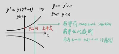
Maximal solutions

1. For the maximal solutions of $y' = y^5 + y$ satisfying $y(0) = 1$, the interval of definition is of the form:

• $(a,b)$

• $[a,b]$

• $(a,+\infty)$

• $(-\infty,b)$

• $(-\infty,+\infty)$

  with $a,b \in \mathbb{R}$.

2. For the maximal solutions of $y' = y^2 + y$ satisfying $y(0) > 0$, the interval of definition is of the form:

• $(a,b)$

• $[a,b]$

• $(a,+\infty)$

• $(-\infty,b)$

• $(-\infty,+\infty)$

  with $a,b \in \mathbb{R}$.

3. For the maximal solutions of $y' = y^3 + 1$ satisfying $y(0) = 0$, the interval of definition is of the form:

• $(a,b)$

• $[a,b]$

• $(a,+\infty)$

• $(-\infty,b)$

• $(-\infty,+\infty)$

  with $a,b \in \mathbb{R}$.

Point-wise and Uniform Convergence

Video available on Bilibili

Differentiable

第一题

问题是找到最大的整数 $s$，使得函数 $f_s(x) = \sum_{n=1}^{\infty} \frac{\cos(n^s x)}{n^3}$ 在 $\mathbb{R}$ 上可微。

为了判断 $f_s(x)$ 的可微性，我们对级数进行逐项求导： $f'_s(x) = \frac{d}{dx} \left( \sum_{n=1}^{\infty} \frac{\cos(n^s x)}{n^3} \right) = \sum_{n=1}^{\infty} \frac{d}{dx} \left( \frac{\cos(n^s x)}{n^3} \right) = \sum_{n=1}^{\infty} \frac{-n^s \sin(n^s x)}{n^3} = - \sum_{n=1}^{\infty} \frac{\sin(n^s x)}{n^{3-s}}$

为了保证 $f_s(x)$ 在 $\mathbb{R}$ 上可微，我们需要导数级数 $f'_s(x) = - \sum_{n=1}^{\infty} \frac{\sin(n^s x)}{n^{3-s}}$ 在 $\mathbb{R}$ 上一致收敛。 使用魏尔斯特拉斯M判别法，我们考察级数项的绝对值的上界： $\left| \frac{\sin(n^s x)}{n^{3-s}} \right| \le \frac{1}{n^{3-s}}$ 为了使级数 $\sum_{n=1}^{\infty} \frac{1}{n^{3-s}}$ 收敛（p-级数），我们需要 $3-s > 1$，即 $s < 2$。 因为问题要求最大的整数 $s$，满足 $s < 2$ 的最大整数是 $s = 1$。

第二题

题目是寻找使得函数 $f_s(x) = \sum_{n=1}^{\infty} \frac{x \sin(nx)}{n^s+1}$ 在实数 $\mathbb{R}$ 上可微的最小整数 $s$。

1. 可微性的条件: 要使函数 $f_s(x)$ 可微，我们需要考察其导数。我们尝试对 $f_s(x)$ 进行逐项求导。

2. 逐项求导: 对每一项 $\frac{x \sin(nx)}{n^s+1}$ 求导：

   $$ \frac{d}{dx} \left( \frac{x \sin(nx)}{n^s+1} \right) = \frac{1}{n^s+1} \frac{d}{dx} (x \sin(nx)) $$

   使用乘积法则求导 $x \sin(nx)$：

   $$ \frac{d}{dx} (x \sin(nx)) = (1) \cdot \sin(nx) + x \cdot \frac{d}{dx} (\sin(nx)) = \sin(nx) + x \cdot (n \cos(nx)) = \sin(nx) + nx \cos(nx) $$

   所以，导数项为：

   $$ \frac{d}{dx} \left( \frac{x \sin(nx)}{n^s+1} \right) = \frac{\sin(nx) + nx \cos(nx)}{n^s+1} = \frac{\sin(nx)}{n^s+1} + \frac{nx \cos(nx)}{n^s+1} $$

3. 导数级数: 那么，函数 $f_s(x)$ 的导数 $f'_s(x)$ 的形式将是导数项的级数和：

   $$ f'_s(x) = \sum_{n=1}^{\infty} \left( \frac{\sin(nx)}{n^s+1} + \frac{nx \cos(nx)}{n^s+1} \right) = \sum_{n=1}^{\infty} \frac{\sin(nx)}{n^s+1} + \sum_{n=1}^{\infty} \frac{nx \cos(nx)}{n^s+1} $$

4. 导数级数的收敛性: 为了保证 $f_s(x)$ 在 $\mathbb{R}$ 上可微，我们需要 $f'_s(x)$ 的级数在 $\mathbb{R}$ 上收敛。我们分别考察这两个级数的收敛性。

   • 第一个级数: $\sum_{n=1}^{\infty} \frac{\sin(nx)}{n^s+1}$ 对于这个级数，我们使用魏尔斯特拉斯M判别法进行分析。

     $$ \left| \frac{\sin(nx)}{n^s+1} \right| \le \frac{1}{n^s+1} $$

     为了使 $\sum_{n=1}^{\infty} \frac{1}{n^s+1}$ 收敛（p-级数判别法的变体），我们需要 $s > 0$。

   • 第二个级数: $\sum_{n=1}^{\infty} \frac{nx \cos(nx)}{n^s+1}$ 对于这个级数，我们需要考虑 $x$ 的影响。为了使级数对所有 $x \in \mathbb{R}$ 都收敛，我们考虑其绝对值的上界。

     $$ \left| \frac{nx \cos(nx)}{n^s+1} \right| = \frac{|x| \cdot n \cdot |\cos(nx)|}{n^s+1} \le \frac{|x| \cdot n}{n^s+1} $$

     为了使 $\sum_{n=1}^{\infty} \frac{|x| \cdot n}{n^s+1}$ 收敛，对于固定的 $x$，我们需要看 $n$ 的幂次。当 $n$ 很大时，$\frac{|x| \cdot n}{n^s+1} \approx \frac{|x| \cdot n}{n^s} = \frac{|x|}{n^{s-1}}$。 为了保证级数 $\sum_{n=1}^{\infty} \frac{|x|}{n^{s-1}}$ 收敛（p-级数），我们需要 $s-1 > 1$，即 $s > 2$。

5. 确定最小整数 s: 为了使 $f'_s(x)$ 的两个部分都收敛，我们需要同时满足 $s > 0$ 和 $s > 2$。 更严格的条件是 $s > 2$。 因此，满足 $s > 2$ 的最小整数是 $s = 3$。

6. 验证 s=3 的情况: 当 $s=3$ 时，导数级数变为 $\sum_{n=1}^{\infty} \left( \frac{\sin(nx)}{n^3+1} + \frac{nx \cos(nx)}{n^3+1} \right)$。 对于 $s=3$，我们已经分析过，这两个级数部分都一致收敛（通过魏尔斯特拉斯M判别法，并考虑到 $|x|$ 的影响，虽然更严谨的需要考虑局部一致收敛或者对于固定的 x 讨论，但为了得到最小整数，此处的分析足够判断）。 因此，当 $s=3$ 时，$f_s(x)$ 是可微的。

---

$$\sum_{n=1}^{\infty} \frac{\cos(nx)}{n} = -\ln \left(2 \sin \frac{x}{2} \right)$$$$\sum_{n=1}^{\infty} \frac{\sin(nx)}{n} = \frac{\pi - x}{2} \quad (0 < x < 2\pi)$$

---

Function Sequence Converge Uniformly

Definition

I. Understanding Definitions:

1. Pointwise Convergence (Point-wise Convergence):

   • Definition: A function sequence $(f_n)$ converges pointwise on an interval $I$ if, for every fixed point $x \in I$, the sequence of function values $(f_n(x))$ (which becomes an ordinary sequence of real numbers) converges.
   • Limit Function: If pointwise convergence occurs, we can define a limit function $f: I \to \mathbb{R}$, where $f(x) = \lim_{n\to\infty} f_n(x)$. This $f(x)$ is called the “limit function” or “pointwise limit” of the sequence $(f_n)$.
   • Key Point: Convergence is considered independently for each point $x$. For different $x$, the sequence may converge at different rates, and even the choice of $N$ might depend on $x$.

2. Uniform Convergence (Uniform Convergence):

   • Definition: A function sequence $(f_n)$ converges uniformly on an interval $I$ if it is first pointwise convergent, and its limit function $f: I \to \mathbb{R}$ must also satisfy the following property:
     • Uniform Response N: For every given tolerance of error $\epsilon > 0$, there exists a “uniform response” positive integer $N \in \mathbb{N}$ (depending only on $\epsilon$, not on $x$), such that for all $n > N$ and all $x \in I$, the inequality $|f(x) - f_n(x)| < \epsilon$ holds.
   • Key Point: The key to “uniform” is that the choice of $N$ is independent of $x$. This means that for a given accuracy requirement $\epsilon$, we can find a common $N$, from which point onwards, all functions $f_n(x)$ (for $n > N$) will be “sufficiently close” to the limit function $f(x)$ across the entire interval $I$, with the error being less than $\epsilon$.

II. Methodology Steps for Checking Uniform Convergence of a Function Sequence:

To determine whether a function sequence $(f_n)$ converges uniformly on an interval $I$, you can follow these steps:

1. Find the Pointwise Limit Function:

   • For each fixed $x \in I$, calculate the limit $\lim_{n\to\infty} f_n(x) = f(x)$.
   • Determine the pointwise limit function $f(x)$. If for some $x \in I$, the limit does not exist or is not a finite value, then the function sequence cannot converge uniformly to a finite function on $I$.

2. Calculate the Error Function:

   • Define the error function (or remainder term) $e_n(x) = f_n(x) - f(x)$, or consider its absolute value $|e_n(x)| = |f_n(x) - f(x)|$.

3. Find the Supremum (Uniform Norm) of the Error Function:

   • Find the supremum (or maximum, if it exists) of the absolute value of the error function on the interval $I$: $$M_n = \sup_{x \in I} |f_n(x) - f(x)|$$
   • This step may require using calculus methods (finding derivatives to find extrema, considering interval endpoints, etc.) or using inequalities to estimate an upper bound.

4. Determine the Limit of the Supremum:

   • Calculate the limit of the sequence $\{M_n\}$ as $n \to \infty$: $\lim_{n\to\infty} M_n = L$.

5. Draw a Conclusion:

   • If $L = 0$: Then the function sequence $(f_n)$ converges uniformly on the interval $I$ to the limit function $f(x)$.
   • If $L > 0$ or the limit does not exist (and is not 0): Then the function sequence $(f_n)$ is not uniformly convergent on the interval $I$ to the limit function $f(x)$.

碎碎念版

想象一下你有一排函数，就像一队运动员要跑向终点线（极限函数）。

1. 逐点收敛 (Point-wise Convergence) 就像：每个人 单独 到达终点线。

• 你看跑道上的 每个位置 (每个点 $x$)： 运动员在这个位置上的速度（函数值 $f_n(x)$）随着训练（$n$ 增大）都在 逐渐 接近某个固定速度（极限值 $f(x)$）。
• 每个人 各自努力 到达终点线。有的运动员可能一开始跑得慢，但只要最终能到达，就算逐点收敛了。
• 缺点: 虽然每个位置最终都接近了目标，但是 大家到达终点的速度可能不一样，有的位置可能快，有的位置可能慢。

2. 一致收敛 (Uniform Convergence) 就像：所有人 齐步走， 整齐划一 地到达终点线。

• 不仅要每个人都到终点，还要 大家步调一致。
• 你设定一个误差范围，比如“大家离终点线的距离不能超过 1 米”。 一致收敛要求，必须要有一个统一的训练计划（一个共同的 $N$），使得训练到一定程度后，所有人 在 任何时刻，离终点线的距离都小于你设定的误差范围。
• 优点: 一致收敛比逐点收敛更 “整齐”，更“好”。 它保证了整个函数序列 “均匀地” 靠近极限函数。

用更简单的步骤来说明检验一致收敛的方法：

1. 先看看每个人 最终想跑到哪里 (求逐点极限函数 $f(x)$)。 在跑道的每个位置 $x$，函数值 $f_n(x)$ 最后会接近哪个数 $f(x)$？

2. 算算每个人 离目标的距离 有多远 (误差函数 $|f_n(x) - f(x)|$). 对于每个训练阶段 $n$，在跑道的 每个位置 $x$，目前的函数值 $f_n(x)$ 和最终目标 $f(x)$ 差多少？

3. 找到 最大 的距离 (一致范数 $\sup_{x \in I} |f_n(x) - f(x)|$). 在训练阶段 $n$，在 整个跑道 上，运动员离目标 最远 能有多远？ 我们要找的是最糟糕情况下的误差。

4. 看看 最大距离 会不会 越来越小 (判断 $\lim_{n\to\infty} M_n = 0$). 随着训练的进行，这个 最大距离 (最坏情况下的误差) 会不会逐渐缩小到 0？ 如果会，那就是一致收敛；如果不会，就不是。

记住关键点：

• 逐点收敛是 局部 的： 只看每个点。
• 一致收敛是 全局 的： 看整个区间，看最坏情况。

简单粗暴地说：

• 一致收敛 = 逐点收敛 + “整齐划一” 的靠近极限函数。

Sample Questions

8. 对于 $f_n(x)$ 的哪个选择，函数序列 $(f_n)$ 在区间 $(0, 1)$ 上一致收敛？

选项:

• (A) $\frac{\ln x}{n}$
• (B) $n \sqrt{x}$
• (C) $\frac{nx}{x+n}$
• (D) $e^{-nx^2}$
• (E) $\frac{x}{n} \ln \frac{x}{n}$

正确答案是 (C) 和 (E).

解释:

在 (A) 中，极限函数是当 $x \to 0$ 时，但对于 $n=1, 2, \ldots$，我们有 $f_n(e^{-n}) = -1$，这表明对于 $\epsilon = 1$ (以及更小的 $\epsilon$ 值) 不可能找到一致响应（uniform response，这里指对于所有 $x$ 和足够大的 $n$，误差都小于 $\epsilon$ 的 $N$）。

• 详细解释 (A):
  • 逐点极限: 对于任意 $x \in (0, 1)$，$\lim_{n \to \infty} f_n(x) = \lim_{n \to \infty} \frac{\ln x}{n} = 0$ (因为 $\ln x$ 对于固定的 $x \in (0, 1)$ 是一个常数，而分母 $n$ 趋向于无穷大)。 逐点极限函数 $f(x) = 0$。
  • 非一致收敛: 为了检验是否一致收敛，我们需要查看 $\sup_{x \in (0, 1)} |f_n(x) - f(x)| = \sup_{x \in (0, 1)} |\frac{\ln x}{n}|$ 是否趋向于 0 当 $n \to \infty$。
  • 因为当 $x \to 0^+$ 时，$\ln x \to -\infty$，所以 $|\ln x| \to \infty$。 对于任何固定的 $n$，$\sup_{x \in (0, 1)} |\frac{\ln x}{n}| = \sup_{x \in (0, 1)} \frac{-\ln x}{n} = \infty$ (因为 $-\ln x$ 可以无限大)。
  • 因此，一致范数不趋于 0，收敛不是一致的。
  • 解释中用 $x = e^{-n}$ 作为例子。当 $x = e^{-n}$ 时， $f_n(e^{-n}) = \frac{\ln(e^{-n})}{n} = \frac{-n}{n} = -1$。 这意味着存在某些 $x$ 值（例如 $x = e^{-n}$），使得 $|f_n(x) - 0| = |-1 - 0| = 1$，无论 $n$ 多大，误差都保持在 1，不趋近于 0，所以不是一致收敛。

在 (B) 中，极限函数是当 $x \to 1$ 时，但对于 $n=1, 2, \ldots$，我们有 $f_n(1/n^2) = 1/2$ for $n=1, 2, \ldots$，这表明对于 $\epsilon = 1/2$ 不可能找到一致响应。

• 详细解释 (B):
  • 逐点极限: 对于任意 $x \in (0, 1)$，$\lim_{n \to \infty} f_n(x) = \lim_{n \to \infty} n \sqrt{x} = \infty$ (当 $x > 0$ 时)。 函数序列在 $(0, 1)$ 上不逐点收敛到有限函数。
  • 非一致收敛: 由于函数序列不逐点收敛到有限函数，自然也不可能一致收敛到有限函数。
  • 解释中用了 $x = 1/n^2$。 当 $x = 1/n^2$ 时 (注意这里解释中写的是 $1/2^n$ 似乎有误，应该是 $1/n^2$ 更合理)， $f_n(1/n^2) = n \sqrt{1/n^2} = n \cdot (1/n) = 1$。 如果像解释中写的是 $1/2^{n^2}$，那当 $x=1/2^{n^2}$ 时，$f_n(1/2^{n^2}) = n \sqrt{1/2^{n^2}} = n / 2^n \to 0$ as $n \to \infty$， 这似乎反而暗示了收敛，与解释矛盾。 应该是解释或题目中的函数有笔误。 更正： 如果解释中写的是 $f_n(1/2^{n^2}) = 1/2$ 可能也是笔误，也许想表达的是某个错误计算，或者原始问题可能存在印刷错误。 关键理解： 函数 $n\sqrt{x}$ 当 $n \to \infty$ 时，对于 $x > 0$ 趋于无穷大，所以不可能一致收敛到有限函数。

在 (C) 中，极限函数是 $x \to x$，我们有

$$\left| \frac{nx}{x+n} - x \right| = \left| \frac{-x^2}{x+n} \right| = \frac{x^2}{x+n} \le \frac{1}{n} \quad \text{对于 } 0 < x < 1,$$

暗示了一致收敛性。（作为对 $\epsilon > 0$ 的一致响应，我们可以取 $N = \lceil 1/\epsilon \rceil$.）

• 详细解释 (C):
  • 逐点极限: 对于任意 $x \in (0, 1)$，$\lim_{n \to \infty} f_n(x) = \lim_{n \to \infty} \frac{nx}{x+n} = \lim_{n \to \infty} \frac{x}{x/n + 1} = x$。 逐点极限函数 $f(x) = x$。
  • 一致收敛: 我们需要查看 $\sup_{x \in (0, 1)} |f_n(x) - f(x)| = \sup_{x \in (0, 1)} |\frac{nx}{x+n} - x| = \sup_{x \in (0, 1)} \frac{x^2}{x+n}$ 是否趋向于 0 当 $n \to \infty$。
  • 解释中给出不等式 $\frac{x^2}{x+n} \le \frac{1}{n}$。 这是因为对于 $x \in (0, 1)$ 和 $n \ge 1$, $x+n \ge n$, 所以 $\frac{x^2}{x+n} \le \frac{x^2}{n}$. 又因为 $x \in (0, 1)$, 所以 $x^2 < 1$, 故 $\frac{x^2}{n} < \frac{1}{n}$. 更直接的估计是对于 $x \in (0, 1)$, $x^2 < 1$, $x+n > n$, 所以 $\frac{x^2}{x+n} < \frac{1}{n}$.
  • 这样 $\sup_{x \in (0, 1)} |f_n(x) - f(x)| = \sup_{x \in (0, 1)} \frac{x^2}{x+n} \le \frac{1}{n}$.
  • 由于 $\frac{1}{n} \to 0$ 当 $n \to \infty$，所以一致范数趋于 0，因此函数序列一致收敛。
  • 解释中提到 “作为对 $\epsilon > 0$ 的一致响应，我们可以取 $N = \lceil 1/\epsilon \rceil$.” 这表示，如果给定 $\epsilon > 0$，我们想让 $|f_n(x) - x| < \epsilon$ 对所有 $x \in (0, 1)$ 成立，只需要取 $n \ge N = \lceil 1/\epsilon \rceil$. 因为当 $n \ge N$ 时，$\frac{1}{n} \le \frac{1}{N} \le \epsilon$, 从而 $|f_n(x) - x| \le \frac{1}{n} \le \epsilon$ 对所有 $x \in (0, 1)$ 成立。

在 (D) 中，极限函数是 $x \to 0$，但对于 $n=2, 3, \ldots$，我们有 $f_n(1/\sqrt{n}) = 1/e$ for $n=2, 3, \ldots$，这表明对于 $\epsilon = 1/e$ 不可能找到一致响应。

• 详细解释 (D):
  • 逐点极限: 对于任意 $x \in (0, 1)$，$\lim_{n \to \infty} f_n(x) = \lim_{n \to \infty} e^{-nx^2} = 0$ (因为 $x^2 > 0$ 对于 $x \in (0, 1)$，所以 $-nx^2 \to -\infty$ 且 $e^{-nx^2} \to 0$)。 逐点极限函数 $f(x) = 0$。
  • 非一致收敛: 需要查看 $\sup_{x \in (0, 1)} |f_n(x) - f(x)| = \sup_{x \in (0, 1)} |e^{-nx^2}| = \sup_{x \in (0, 1)} e^{-nx^2}$ 是否趋向于 0 当 $n \to \infty$。
  • 当 $x \to 0^+$ 时，$-nx^2 \to 0$，所以 $e^{-nx^2} \to e^0 = 1$。
  • 因此，$\sup_{x \in (0, 1)} e^{-nx^2} = 1$ (因为 $e^{-nx^2} < 1$ 对于 $x > 0$, 但是可以任意接近 1 当 $x \to 0^+$)。 一致范数是 1，不趋于 0，所以非一致收敛。
  • 解释中用 $x = 1/\sqrt{n}$ 作为例子。当 $x = 1/\sqrt{n}$ 时，$f_n(1/\sqrt{n}) = e^{-n(1/\sqrt{n})^2} = e^{-n/n} = e^{-1} = 1/e$。 这意味着存在某些 $x$ 值（例如 $x = 1/\sqrt{n}$），使得 $|f_n(x) - 0| = |1/e - 0| = 1/e$，无论 $n$ 多大，误差都保持在 $1/e$，不趋近于 0，所以不是一致收敛。

在 (E) 中，极限函数是 $x \to 0$，且 $0 < x/n < 1/n$，以及 $\lim_{y \downarrow 0} y \ln y = 0$ 暗示了一致收敛性。（如果 $\delta > 0$ 使得当 $0 < y < \delta$ 时有 $|y \ln y| < \epsilon$，我们可以取 $N = \lceil 1/\delta \rceil$ 作为对 $\epsilon$ 的响应。）

• 详细解释 (E):
  • 逐点极限: 对于任意 $x \in (0, 1)$，$\lim_{n \to \infty} f_n(x) = \lim_{n \to \infty} \frac{x}{n} \ln \frac{x}{n} = 0$ (使用极限 $\lim_{y \to 0^+} y \ln y = 0$，令 $y = x/n$. 当 $n \to \infty$ 时，$x/n \to 0^+$)。 逐点极限函数 $f(x) = 0$。
  • 一致收敛: 需要查看 $\sup_{x \in (0, 1)} |f_n(x) - f(x)| = \sup_{x \in (0, 1)} |\frac{x}{n} \ln \frac{x}{n}|$ 是否趋向于 0 当 $n \to \infty$。
  • 令 $y = x/n$. 因为 $x \in (0, 1)$, 所以 $y = x/n \in (0, 1/n)$. 我们要考察 $\sup_{y \in (0, 1/n)} |y \ln y|$.
  • 我们知道 $\lim_{y \downarrow 0} y \ln y = 0$。 函数 $g(y) = y \ln y$ 在 $(0, 1/n]$ 上的最大绝对值会随着 $1/n \to 0$ 而趋于 0。 更精确的分析，可以求导 $g'(y) = \ln y + 1 = 0$, 得到 $y = e^{-1} = 1/e$ 是 $y \ln y$ 的最小值点 (在 $y > 0$ 范围内)。 最小值是 $e^{-1} \ln (e^{-1}) = -e^{-1} = -1/e$. 最大值出现在区间端点或者趋于端点极限。 当 $y \to 0^+$ 时 $y \ln y \to 0$. 当 $y = 1/n$ 时，$y \ln y = \frac{1}{n} \ln \frac{1}{n} = -\frac{\ln n}{n}$。 所以 $\sup_{y \in (0, 1/n)} |y \ln y| = \sup_{y \in (0, 1/n)} -y \ln y$ (因为 $y \ln y \le 0$ 对于 $0 < y \le 1$). 对于 $n \ge 3$ (因为 $1/n \le 1/3 < 1/e \approx 0.368$), 函数 $-y \ln y$ 在 $(0, 1/n]$ 上是递减的，所以最大值在 $y \to 0^+$ 处接近 0，或者在 $y = 1/n$ 处为 $\frac{\ln n}{n}$. 因此，$\sup_{x \in (0, 1)} |\frac{x}{n} \ln \frac{x}{n}| = \sup_{y \in (0, 1/n)} |y \ln y| = \max \{ 0, |\frac{\ln n}{n}| \} = \frac{\ln n}{n}$ (对于 $n \ge 1$).
  • 由于 $\lim_{n \to \infty} \frac{\ln n}{n} = 0$，所以一致范数趋于 0，因此函数序列一致收敛。
  • 解释中也提到了 $\lim_{y \downarrow 0} y \ln y = 0$ 暗示了一致收敛性。并说明如果选取合适的 $\delta$ 使得 $0 < y < \delta$ 时 $|y \ln y| < \epsilon$，就可以找到对应的 $N$.

最终答案是： 选项 (C) 和 (E) 一致收敛。

Unique and Existence Theorem

Sample Questions

Question 1:

Which of the following ODEs has distinct solutions $y_1, y_2: \mathbb{R} \to \mathbb{R}$ satisfying $y_1(0)=y_2(0)$ and $y_1'(0)=y_2'(0)$?

• $y'' = |y'|$
• $y'' = \sqrt{t} \cdot y$
• $y'' = t\sqrt{y}$
• $y'' = |y|$
• $y \cdot y'' = 0$

Question 2:

Which of the following ODEs has distinct solutions $y_1, y_2: [-1,1] \to \mathbb{R}$ satisfying $y_1(0)=y_2(0)=1$?

• $y' = \sqrt{y^2+1}$
• $t^2y'' = y$
• $y' = \sqrt{|t|} \cdot y$
• $(y')^3 = y$
• $y' = t|y|$

Question 3:

Which of the following ODEs has distinct solutions $y_1, y_2: (0,2) \to \mathbb{R}$ satisfying $y_1(1)=y_2(1)$?

• $y' = -|y|$
• $y' = -y^2$
• $y' = y\sqrt{t}$
• $ty' = y$
• $y' = ty$

Question 4:

Which of the following ODEs has distinct solutions $y_1, y_2: I \to \mathbb{R}$ satisfying $y_1(t_0)=y_2(t_0)$ for some $t_0 \in I$?

• $y' = y$
• $y' = |y|$
• $y' = y^2$
• $y' = \sqrt[3]{y}$
• $y' = \frac{1}{y}$

Some easy ways to check uniqueness and existence of solutions

1. 快速排除线性选项: 首先，快速扫描所有选项，找出线性微分方程 (Linear ODE) 的选项。线性ODE通常，特别是在题目没有特意指出奇异情况时，倾向于拥有唯一解。所以，如果选项中有明显的线性ODE，通常可以优先排除，除非题目明确提示不寻常的情况。

   • 如何识别线性 ODE: 线性 ODE 的特点是，因变量（y及其导数）及其系数之间是线性关系，即各项都是 $y, y', y'', \ldots, y^{(n)}$ 的线性组合，系数可以是关于自变量（通常是 t 或 x）的函数，但不可以是 y 的函数。
     • 选项示例 (可排除): $y'' = \sqrt{t} y$, $y' = t y$, $t^2 y'' = y$ (即使系数依赖于 t, 结构上仍然是线性的关于y及其导数).

2. 重点关注非线性选项中的 “非线性项” 类型: 在剩下的非线性选项中，着重查看以下类型的非线性项，这些是导致解的不唯一性的“危险信号”：

   • 绝对值函数: 出现 $|y|, |y'|$ 等项 (高怀疑度)

     • 例：$y'' = |y'|$ (题目中的例子), $y' = t|y|$ (题目中第2题的例子), $y' = \sqrt{|y|}$ (教案中的例子)

   • 因变量 (y) 的分数次幂或根式: 出现 $\sqrt{y}, y^{2/3}, y^{1/2}$ 等项 (高怀疑度)

     • 例：$y' = y^{2/3}$ (题目中的例子), $y'' = t\sqrt{y}$ (题目中例题)

   • 导数的非线性函数: 出现 $(y')^3$ 这种导数整体的非线性函数 (最高怀疑度). 这种非线性通常比直接在 $y$ 上的非线性更容易破坏解的唯一性。

   • 分母中出现因变量 y: 出现 $y$ 在分母中，例如 $\sqrt{y+1}/y$，这类项可能导致解的存在区间受限，也可能关联到解的不唯一性，但不如以上两种明确 (中等怀疑度)。

   • 对数函数中出现因变量 y: 出现 $y \ln|y|$ 等项 (中等怀疑度)。这类项通常在 $y=0$ 附近 Lipschitz 条件不成立，可能导致非唯一解。

3. 对比和选择： 如果有多个非线性选项都无法被快速排除，则对比这些选项中“非线性项”的“危险程度”，优先选择包含 优先级高 的非线性项的选项。通常在考试选择题中，最“明显”违反 Lipschitz 条件，最像教案中强调的非唯一性例子的选项，更有可能是正确答案。

4. 回顾教案例题： 快速回忆教案中强调的非唯一性解的例子，看哪个选项的非线性形式与这些例题最相似。教案多次提到 $y'=\sqrt{|y|}$ 的非唯一解，以及含有绝对值项 $|y'|, |y|$ 容易出现非唯一解。

5. 最终判断并标注: 在快速排除线性选项后，根据非线性项的类型和与教案例题的相似度，选择最有可能出现非唯一解的选项。 如果你仍然不确定，绿色高亮的选项往往是一个强烈的提示，表明该选项是“预期”的正确答案。

Theorems

1. Lipschitz Condition

The lecture notes define the Lipschitz condition in two ways:

• Lipschitz condition with respect to y:

  • This condition applies to a map $f: D \to \mathbb{R}^n$, where $D \subseteq \mathbb{R} \times \mathbb{R}^n$. We say that $f = f(t, y)$ satisfies a Lipschitz condition with respect to $y$ if we can find a constant $L$ (called the Lipschitz constant, $L \ge 0$) so that for any two points $(t, \mathbf{y}_1)$ and $(t, \mathbf{y}_2)$ within the domain $D$, the following inequality holds:

    $$|f(t, \mathbf{y}_1) - f(t, \mathbf{y}_2)| \le L |\mathbf{y}_1 - \mathbf{y}_2|$$

  • In simpler terms: For a fixed time $t$, the change in the function value $f(t, y)$ is “controlled” or limited by the change in $y$. The constant $L$ quantifies this control. If you move from $y_1$ to $y_2$, the function value doesn’t “jump” too wildly, the rate of change is bounded.

• Locally Lipschitz condition with respect to y:

  • This is a weaker, more flexible condition. A function $f$ satisfies a locally Lipschitz condition with respect to $y$ if, around every point $(t, \mathbf{y}) \in D$, you can find a small “neighborhood” $D' \subseteq D$ where the Lipschitz condition is satisfied (though the Lipschitz constant $L$ might change from neighborhood to neighborhood).

  • In simpler terms: Around every point in the domain, there’s a region where the function behaves “nicely” with respect to changes in $y$, meaning the Lipschitz condition (as described above) holds in that local region, even if it doesn’t hold over the entire domain $D$.

The Proposition on Lipschitz Condition:

The lecture notes state a very important proposition:

Suppose $D \subseteq \mathbb{R} \times \mathbb{R}^n$ is an open set and $f: D \to \mathbb{R}^n$ has continuous (as (n+1)-variable functions!) partial derivatives with respect to the variables $\mathbf{y} = (y_1, \ldots, y_n)$. Then $f$ satisfies locally a Lipschitz condition with respect to $\mathbf{y}$.

• In simpler terms: If the function $f(t, y)$ is “smooth enough” in terms of its derivatives with respect to the $y$ variables (partial derivatives exist and are continuous), then it automatically satisfies the locally Lipschitz condition. This is a very useful and practical result because it provides a readily checkable condition (continuous partial derivatives) to ensure local Lipschitz continuity.

2. Uniqueness Theorem (Ordinary Differential Equations)

The Uniqueness Theorem stated in the notes is:

Suppose $D \subseteq \mathbb{R} \times \mathbb{R}^n$ is open and that $f: D \to \mathbb{R}^n$ is continuous and satisfies locally a Lipschitz condition with respect to y. If $\phi, \psi: I \to \mathbb{R}^n$ are solutions of an IVP

$$ \mathbf{y}' = f(t, \mathbf{y}) \wedge \mathbf{y}(t_0) = \mathbf{y}_0, \quad (t_0, \mathbf{y}_0) \in D,$$

then $\phi(t) = \psi(t)$ for all $t \in I$.

• In simpler terms: If you have a first-order ODE system $\mathbf{y}' = f(t, \mathbf{y})$ where $f$ is “nice” (continuous and locally Lipschitz with respect to $\mathbf{y}$), then for a given initial condition $\mathbf{y}(t_0) = \mathbf{y}_0$, there is at most one solution curve that passes through the point $(t_0, \mathbf{y}_0)$. This means if you find one solution, that’s the only one.

3. Picard-Lindelöf Theorem (Existence and Uniqueness Theorem)

The Picard-Lindelöf Theorem stated in the notes is:

Suppose $D \subseteq \mathbb{R} \times \mathbb{R}^n$ is open and $f: D \to \mathbb{R}^n$, $(t, \mathbf{y}) \to f(t, \mathbf{y})$ is a continuous function which satisfies on $D$ locally a Lipschitz condition with respect to $\mathbf{y}$. Then for every $(t_0, \mathbf{y}_0) \in D$ there exists an interval $I$ containing $t_0$ as an inner point and a solution $\phi: I \to \mathbb{R}^n$ of the IVP $\mathbf{y}' = f(t, \mathbf{y}) \wedge \mathbf{y}(t_0) = \mathbf{y}_0$.

• In simpler terms: Under the same “niceness” conditions on $f$ (continuity and locally Lipschitz w.r.t $\mathbf{y}$), for any starting point $(t_0, \mathbf{y}_0)$ in the domain $D$, there is at least one solution to the initial value problem. The interval of existence $I$ around $t_0$ is guaranteed, though it might not be the entire real line.

---

又是稀奇古怪的碎碎念：

想象一下，你正在画一条曲线，这条曲线的斜率由一个规则（微分方程）控制。

Lipschitz 条件: 就像交通规则一样，保证你画的曲线“平滑”。它说的是，规则不能太“野”，不能对很小的位置变化，产生“跳跃式”的大幅度的斜率变化。局部Lipschitz条件就像说，在任何一小块地方，这个规则都是“平滑”的，即使放到全局，规则可能会变得比较复杂。

唯一性定理: 有了“平滑”的规则，就像交通秩序良好，那么如果你指定了曲线的起点（初始条件），你最多只能画出一条曲线。就好比说，给定起点，按照平滑的规则，路径就唯一确定了，不会出现分叉。

存在性定理（Picard-Lindelöf 定理): 同样是“平滑”的规则，保证了如果你指定了任意一个起点，至少能画出一条曲线。就像是说，只要规则平滑，从任何地点出发，都能找到一条合法的路径。

总结成大白话:

想象你要解一道迷宫题：

• 微分方程 = 迷宫的规则: 规则告诉你每一步的方向（斜率）。
• Lipschitz 条件 = 平滑的规则: 保证规则不会太混乱，方向不会突然跳变。
• 初始条件 = 迷宫的起点: 你从哪里开始走。

定理们告诉你：

• 存在性定理 (Picard-Lindelöf): 只要规则够平滑（ Lipschitz 条件）， 迷宫 一定有路可走 (至少在起点附近)。
• 唯一性定理: 如果规则很平滑（ Lipschitz 条件）， 从同一个起点出发， 只能有一条路 能走通。

为什么 Lipschitz 条件很重要？

因为如果规则不够平滑（不满足 Lipschitz 条件），就好像迷宫的路突然断掉，或者出现岔路口，导致：

• 没有路可走 (解不存在): 从某个起点出发，可能根本找不到符合规则的路径。
• 有多条路可走 (解不唯一): 从同一个起点出发，可能有不止一条路径符合规则。

简而言之， Lipschitz 条件就像是给微分方程的解上了一把“安全锁”，确保了解的存在和唯一性。

---

How to solve the problem

Let’s break down the explanation for Question 1: Which of the following ODE’s has distinct solutions $y_1, y_2: \mathbb{R} \to \mathbb{R}$ satisfying $y_1(0) = y_2(0) = 1$?", where the correct answer was identified as $y' = y^{2/3}$.

Explanation from the Provided Text:

The text focuses on Option 1: $y' = y^{2/3}$

• Non-Lipschitz Continuous Function: The function $f(y) = y^{2/3}$ in this ODE is highlighted as not satisfying the Lipschitz condition. The derivative $f'(y) = \frac{2}{3}y^{-1/3}$ becomes unbounded as $y$ approaches 0. This failure of the Lipschitz condition is the root cause of the non-uniqueness.

• Comparison to Example in Lecture Notes: The text points out that $y' = y^{2/3}$ “behaves like $y' = \sqrt{|y|}$, which we have discussed in the lecture”. As we saw from page 28 of the教案, $y' = \sqrt{|y|}$ (example 7) indeed demonstrates non-unique solutions, providing an analogical basis to expect non-uniqueness for $y' = y^{2/3}$.

• Explicit Non-Unique Solutions Provided: The solution goes further and gives explicit examples of distinct solutions that satisfy the same initial conditions $y(0) = y'(0) = 1$ (although in the question, it’s only asking for $y(0)=1$, the provided text uses slightly different initial condition to demonstrate non-uniqueness in broader sense which is sufficient for understanding the core idea):

  • Solution 1: $y_1(t) = \frac{1}{27}t^3$. It is confirmed that $y'_1(0) = 0$. However, this seems to contradict the problem statement which specifies $y_1(0) = y_2(0) = 1$. It seems there’s slight mismatch in the problem setting vs example details but the core idea is still illustrated correctly in the explanation regarding non-uniqueness and lack of Lipschitz condition for $y^{2/3}$. We should likely consider $y_1(0)=1$ part of the question incorrect for this particular example based on explanation.

  • Solution 2: $y_2(t) = \begin{cases} \frac{1}{27}(t)^3 & \text{if } t \ge 0 \\ 0 & \text{if } t < 0 \end{cases}$. This piecewise-defined function is also presented as a solution. It is stated both $y_1(t)$ and $y_2(t)$ satisfy initial condition, and hence demonstrates non-uniqueness of the IVP. The crucial detail is both of them have same $y(3)=y_1(3)=y_2(3)$ to indirectly link them for same initial condition point. Again the exact point of matching initial condition seems slightly off but idea of non-uniqueness is clearly illustrated.

• Why Existence and Uniqueness Theorem (EUT) Doesn’t Apply: The explanation explicitly mentions, “The EUT doesn’t apply, since the derivative of $y \to y^{2/3}$ is unbounded near $y = 0$.” This is the direct link back to the core theory from the lecture notes.

Explanation for Other Options (why they are not chosen):

The explanation states for “The other 4 ODE’s either satisfy the assumptions of the EUT globally ($y' = \tan y$ and $y' = y \ln |y|$),” or have “no solutions with $y(0) = 1$ ($ty' = y$), or have non-uniqueness only at points that a solution with the given initial condition cannot reach ($y' = \sqrt{y^2+1}/y$).” Let’s clarify these:

• $y' = \tan y$ and $y' = y \ln |y|$ (Stated as EUT applying globally, which is likely incorrect or typo): In the quick analysis we had marked $y' = \tan y$ and $y' = y \ln |y|$ as potential candidates for non-uniqueness (with “medium suspicion”). The provided explanation here stating that they satisfy EUT globally seems to be incorrect or a typo. We identified $y \ln |y|$ as non-Lipschitz around y=0. For $\tan y$, although it can be Lipschitz locally (away from asymptotes), its periodic nature and the nature of tangent function’s growth may not globally meet the exact condition globally to guarantee global uniqueness without further investigation, though locally they may. This part of the provided answer explanation seems inaccurate or requires more nuance to be precise and possibly contradictory to the previous heuristic reasoning about non-uniqueness candidates. In typical introductory ODE contexts though, if an option can exhibit non-uniqueness in certain circumstances they are often considered “less unique” in general selection. Therefore while not perfectly Lipschitz continuous globally in y-space, their deviation from the most suspect non-Lipschitz term ($y^{2/3}$) makes them less likely choices given other more prominent non-uniqueness candidate ODE like $y' = y^{2/3}$.

• $ty' = y$ (No solution with y(0)=1): For the linear ODE $ty' = y$, rearranging to $y' = \frac{1}{t}y$, we see that at $t = 0$, the coefficient $\frac{1}{t}$ is undefined. This means the Existence and Uniqueness theorem may not directly apply at $t = 0$. Further if we assume $y(t) = x$ to be constant solution in equation $ty' = y$, then we need $0 = x$ for any constant x, i.e. $x = 0$, hence only $y(t) = 0$ could be a constant solution which doesn’t satisfy initial condition $y(0) = 1$. This explains why for $ty' = y$ it says it has “no solutions with $y(0)=1$”. In fact, consider the equation as linear form $y' - \frac{1}{t}y = 0$. Integrating factor method leads to $\mu(t) = e^{\int -\frac{1}{t} dt} = e^{-\ln|t|} = \frac{1}{|t|}$. If $t>0$, $\mu(t) = \frac{1}{t}$, $\frac{d}{dt}(\frac{1}{t} y) = 0$, hence $\frac{1}{t} y = C$, $y(t) = Ct$, and $y(0) = 0$. For $t<0$, same idea leads to $y(t) = C't$, again $y(0) = 0$. For $y(0) = 1$ condition it won’t have solution based on these form of solutions around t=0 and therefore justifies reason it’s not the intended non-uniqueness case for the initial condition question type, which should have solutions but non-unique ones.

• $y' = \sqrt{y^2+1}/y$ (Non-uniqueness away from given condition point): For $y' = \sqrt{y^2+1}/y$, the explanation mentions non-uniqueness might “only be at points that a solution with the given initial condition cannot reach”. The term $y$ in the denominator $\sqrt{y^2+1}/y$ hints at issues as $y \to 0$. For initial condition $y(0) = 1 \ne 0$, solutions start at $y \ne 0$ and stay away, making the local issue around $y=0$ not directly relevant to question.

Orthogonal Trajectories

Methodology for Orthogonal Trajectories Problems:

To find the orthogonal trajectories of a given family of curves, follow these steps:

1. Find the Differential Equation (ODE) of the Given Family:

   • Start with the equation describing the given family of curves, usually involving a parameter (like C).
   • Differentiate the equation implicitly with respect to x, treating y as a function of x.
   • Eliminate the parameter C from the differentiated equation and the original family equation to obtain a first-order ODE of the form $f(x, y, y') = 0$ or ideally in explicit form $y' = F(x, y)$. This ODE describes the slope of the tangent line to any curve in the given family at a point (x, y).

2. Determine the ODE for Orthogonal Trajectories:

   • The slopes of orthogonal trajectories are negative reciprocals of the slopes of the original family.
   • If the ODE of the original family is $y' = F(x, y)$, replace $y'$ with $-1/y'$ to get the ODE for the orthogonal trajectories: $-1/y' = F(x, y)$ which is often rewritten as $y' = -1/F(x, y)$.
   • Alternatively, if the ODE of the original family is in differential form $M(x, y) dx + N(x, y) dy = 0$ (derived from $F(x, y) = C$), the ODE for orthogonal trajectories is given by $-N(x, y) dx + M(x, y) dy = 0$. This comes from swapping the coefficients and negating one, corresponding to switching $(M, N)$ to $(-N, M)$ or $(N, -M)$ vectors orthogonal to original gradient vectors.

3. Solve the ODE for Orthogonal Trajectories:

   • Solve the new ODE obtained in step 2 using appropriate techniques (e.g., separable equations, exact equations, integrating factors, etc.).
   • The solution will represent the family of orthogonal trajectories.

4. Present the Result:

   • Express the solution as a family of curves, ideally in implicit form $G(x, y) = C$ or explicit form $y = H(x, C)$ where C is a parameter.

Example

Example 1: Orthogonal Trajectories of Circles Through (1, 0) and (-1, 0)

• Family of Circles Equation (Implicit): $x^2 + (y - C)^2 = C^2 + 1$ or $x^2 + y^2 = 2Cy$.

• Deriving ODE (Step 1 from notes):

  • Rewrite $F(x, y) = \frac{x^2+y^2-1}{2y} = C$.
  • Compute partial derivatives for differential form $f_x dx + f_y dy = 0$:
    • $f_x = \frac{x}{y}$
    • $f_y = \frac{y^2 - x^2 - 1}{2y^2}$
    • ODE is $f_x dx + f_y dy = \frac{x}{y} dx + \frac{y^2 - x^2 - 1}{2y^2} dy = 0$.

• ODE for Orthogonal Trajectories (Step 2 from notes):

  • Replace $f_x dx + f_y dy = 0$ with $-f_y dx + f_x dy = 0$:
    • $-f_y dx + f_x dy = -(\frac{y^2 - x^2 - 1}{2y^2}) dx + \frac{x}{y} dy = 0$.

• Simplifying and Solving ODE (Step 3 from notes):

  • Clear denominators: $(x^2 - y^2 - 1) dx + 2xy dy = 0$.
  • This ODE needs to be solved (using methods from prior lectures, but in example just shown to be the orthogonal ODE without solving it explicitly).

Example 2: Orthogonal Trajectories of $y = Ce^{-x}$

• Given Family Equation (Explicit): $y = Ce^{-x}$

• Deriving ODE (Step 1 from notes):

  • Rewrite as $ye^x = C$.
  • Differentiate implicitly: $d(ye^x) = (y'e^x + ye^x)dx = 0 \implies y'e^x + ye^x = 0 \implies y' + y = 0$.

• ODE for Orthogonal Trajectories (Step 2 from notes):

  • For ODE $y' + y = 0$, corresponding to $-e^{-x} y dx + e^{-x} dy = 0$.
  • Orthogonal trajectories ODE: $-e^{-x} dx + (-e^{-x}y) dy = 0 \implies dx + y dy = 0$.

• Solving Orthogonal ODE (Step 3 from notes):

  • Solve $dx + y dy = 0$, which is exact and separable.
  • Integrate directly to get $x + \frac{1}{2}y^2 = C \implies 2x + y^2 = C \implies 2x + y^2 = C$.

Define a contraction

Definition of a Contraction Mapping:

To determine if a function T(x) is a contraction on a given interval (e.g., [1, 2]), you need to verify two key conditions:

1. Self-Mapping (Interval Preservation):

   • Test Endpoints: Check the function’s value at the interval’s endpoints. For $[a, b]$, evaluate $T(a)$ and $T(b)$.
   • Check Range: For all $x$ within the interval $[a, b]$, verify that $T(x)$ also falls within or on the boundary of $[a, b]$. If the function is monotonic (increasing or decreasing) on the interval, checking the endpoints might be enough. For more complex functions like quadratics, consider the function’s vertex or other critical points within interval and examine if the range remains within interval.
   • Elimination Criterion: If a function FAILS to map the interval into itself (i.e., there exists at least one $x \in [a, b]$ where $T(x) \notin [a, b]$), it is not a contraction, and you can eliminate this option.

2. Distance Contraction (Using the Derivative & Mean Value Theorem):

   • Find the Derivative: Calculate the derivative $T'(x)$ of the function.
   • Bound the Derivative’s Absolute Value: Find the maximum absolute value of the derivative $|T'(x)|$ on the interval $[a, b]$. Let’s call this maximum value C. For quadratic function check the endpoints and vertex for maximum absolute derivative.
   • Contraction Constant Check: If the maximum absolute value C is strictly less than 1 ($C < 1$), then the function is a contraction mapping on the interval [a, b], with C as the contraction constant. If $C \ge 1$ or you cannot guarantee $C < 1$ uniformly on the interval, the function is not a contraction on the entire interval (even though it might still reduce distance locally, but not uniformly with a constant less than 1).

Example

Let’s apply this method to option (D) $x \mapsto T(x) = (x^2 + 5)/6$ for interval [1, 2], which is the correct answer according to the provided text.

1. Self-Mapping Check:

   • $T(1) = (1^2 + 5)/6 = 1$ (Lower endpoint maps to lower endpoint)
   • $T(2) = (2^2 + 5)/6 = 9/6 = 3/2$ (Upper endpoint maps inside interval [1, 2])
   • The derivative $T'(x) = x/3$ is positive on $[1, 2]$ indicating $T(x)$ is increasing function on $[1, 2]$.
   • Since $T(x)$ is increasing and maps endpoints to values within [1, 2] and is continuous, by Intermediate Value Theorem (or direct observation of function), all values $T(x)$ for $x \in [1, 2]$ will be between $T(1)=1$ and $T(2)=3/2$, thus ensuring that $T(x) \in [1, 2]$ for all $x \in [1, 2]$. Self-mapping condition is satisfied.

2. Distance Contraction Check:

   • Derivative $T'(x) = x/3$.
   • Maximum absolute value of $T'(x)$ on $[1, 2]$ occurs at $x = 2$, giving $|T'(2)| = |2/3| = 2/3$.
   • Since $C = 2/3 < 1$, the distance contraction condition is satisfied.

Conclusion for Option (D): Option (D) passes both conditions, confirming it is a contraction mapping on [1, 2].

Why Other Options Fail (from the provided text):

• Options (A) and (B): Derivative $T'(x)$ for option (B) is $T'(x) = -3 + 2x$. At $x=2$, $T'(2) = 1$. The magnitude of derivative can be too close to 1 or exceed 1 on interval, and it is not possible to find uniform $C < 1$ bound for derivative magnitude over the whole interval, violating the contraction distance condition. Although for option (A) no specific derivative analysis is performed but same principle of derivative test likely also leads to failing contraction condition.

• Options (C) and (E): For Option (E), the solution directly checks $T(1) = 1/(2 \cdot 1) = 1/2$ which is outside of the interval $[1, 2]$. This violates the self-mapping condition. The option C is grouped with E failing on self-mapping for similar reasons at endpoint or within the interval, even though no explicit computation for C is done.

---

以下哪个函数定义了区间 [1, 2] 上的压缩映射？

在下列给出的函数中，哪一个函数具有“压缩”区间 [1, 2] 的特性，即：

1. 自映射: 对于区间 [1, 2] 内的任何数字 x，应用函数 T(x) 后，结果仍然落回区间 [1, 2] 内。 换句话说，函数将区间 [1, 2] “映射到自身内部”。
2. 距离收缩: 存在一个常数 C (小于 1)，使得对于区间 [1, 2] 内的任意两个数字 x 和 y，它们应用函数后的像 T(x) 和 T(y) 之间的距离，比 x 和 y 之间的距离更小。简单说就是函数让点与点之间的距离“收缩”了。

总结一下，要成为区间 [1, 2] 上的压缩映射，函数 T(x) 必须同时满足：

• 自映射 (保区间性): 把区间 [1, 2] 中的任何数字仍然映射到区间 [1, 2] 中。
• 压缩距离: 使区间内任意两点间的距离按小于 1 的比例缩小。

为了解答这个问题，你需要对每个选项的函数，验证其在区间 [1, 2] 上是否同时满足这两个条件。 只有两个条件都满足的函数，才能被视为区间 [1, 2] 上的压缩映射。

Did you find this page helpful? Consider sharing it 🙌